What is time series forecasting?

Time series forecasting is the process of predicting future values based on past observations. It's widely used in fields like weather prediction, stock market analysis, sales forecasting, and even cryptocurrency trends like Bitcoin and Ethereum.

A commonly used model for time series forecasting is the ARIMA model which stands for AutoRegressive Integrated Moving Average and is represented as

$$
\text{ARIMA}(p, d, q)
$$

Where:
- \( p \) is the order of the autoregressive (AR) part,  
- \( d \) is the degree of differencing (to make the series stationary),  
- \( q \) is the order of the moving average (MA) part.

The mathematical formulation of the ARIMA model is

$$
y'_t = c + \sum_{i=1}^{p} \phi_i y'_{t-i} + \sum_{i=1}^{q} \theta_i \varepsilon_{t-i} + \varepsilon_t
$$

Where:
- \( y'_t \) is the differenced time series (after applying differencing \( d \) times),
- \( \phi_i \) are the autoregressive coefficients,
- \( \theta_i \) are the moving average coefficients,
- \( \varepsilon_t \) is the error term (white noise),
- \( c \) is a constant.
 

In this article, I would like to show you how to use time series forecasting to implement reading and displaying Bitcoin (BTC) time series data using the autoregressive integrated moving average (ARIMA) model.

Implementation

I will start by reading the historical prices for BTC using the Pandas data reader and yfinance libraries. But first, let’s install it using a pip command in the terminal.

pip install pandas-datareader
pip install yfinance

import Packages

Let’s import the whole library itself and relax the display limits on columns and rows:

import pandas_datareader.data as pdr
from statsmodels.tsa.arima.model import ARIMA
import datetime
import pandas as pd 
import matplotlib.pyplot as plt
import seaborn as sns
import yfinance as yfin
import numpy as np
from sklearn.metrics import mean_squared_error



yfin.pdr_override()
pd.set_option('display.max_columns', None)
pd.set_option('display.max_rows', None)
sns.set()yfin.pdr_override()
pd.set_option('display.max_columns', None)
pd.set_option('display.max_rows', None)
sns.set()start_date = '2021-01-01'
end_date = datetime.datetime.now()
btc_price= pdr.get_data_yahoo(['BTC-USD'],start_date,end_date)

btc_price.head()# let select the column Close: The last price at which BTC was purchased on that day
btc_price = btc_price[['Close']]
# save it as csv file
btc_price.to_csv("btc.csv")btc_df = pd.read_csv("btc.csv")
btc_df.rename(columns = {'Close':'BTC-USD'}, inplace = True)
btc_df.index = pd.to_datetime(btc_df['Date'], format='%Y-%m-%d')
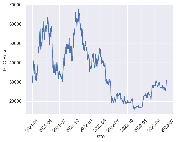
btc_df.head()

Plotting

plt.ylabel('BTC Price')
plt.xlabel('Date')
plt.xticks(rotation=45)

plt.plot(btc_df.index, btc_df['BTC-USD])

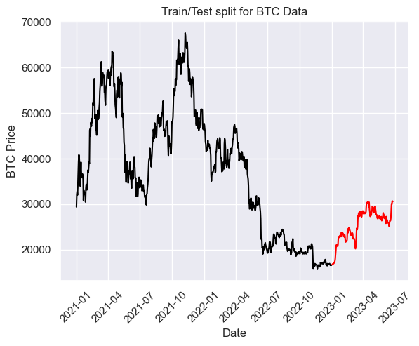
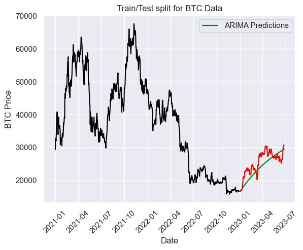
Train/test split

train = btc_df[btc_df.index < pd.to_datetime("2023-1-1", format='%Y-%m-%d')]
test = btc_df[btc_df.index > pd.to_datetime("2023-1-1", format='%Y-%m-%d')]

plt.plot(train, color = "black")
plt.plot(test, color = "red")
plt.ylabel('BTC Price')
plt.xlabel('Date')
plt.xticks(rotation=45)
plt.title("Train/Test split for BTC Data")
plt.show()

Model

# output y
y = train['BTC-USD']

model = ARIMA(y, order = (1,0,1))
model = model.fit()y_pred = model.get_forecast(len(test.index))
y_pred_df = y_pred.conf_int(alpha = 0.05) 
y_pred_df["Predictions"] = model.predict(start = y_pred_df.index[0], end = y_pred_df.index[-1])
y_pred_df.index = test.index
y_pred_df.hea()

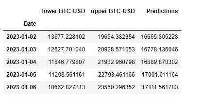
y_pred_out = y_pred_df["Predictions"] 
plt.plot(train, color = "black")
plt.plot(y_pred_out, color='green', label = 'ARIMA Predictions')
plt.plot(test, color = "red")
plt.ylabel('BTC Price')
plt.xlabel('Date')
plt.xticks(rotation=45)
plt.title("Train/Test split for BTC Data")
plt.legend()

means squared error

arma_rmse = np.sqrt(mean_squared_error(test["BTC-USD"].values, y_pred_df["Predictions"]))
print("RMSE: ",arma_rmse)

output:
  RMSE:  2573.424351673843